Please, if you find any errors, contact me. I’ll be glad to hear from you and learn some more :]
- The nearest neighbor rule
- Characteristics
- Does it work?
- Visualizations
- Distance Metrics
- Shortcommings
- Curse of dimensionality on KNN
This is a technique from the beginnings of learning algorithms as a way to apply a rule to classification problems. It’s was first formalized by Cover and Hart in 1967, nevertheless already practiced in many domains, it’s based on the simple premise that neighbors can tell a lot about the class of an unknown point. In practical terms, one can use the nearest neighbors as a decision rule to assign an unknown input to the class of its nearest neighbor in a procedure that independents of the distribution of the samples.
The nearest neighbor rule
- Given an new input x’
- An set of points {x1, θ1} … {xn, θn} where θ represents the class.
- And dist a distance metric
- The nearest neighboor of x’ is:
min(dist(x1, x)) == dist(xn', x)- The nearest neighboor is, from all points, the point who has the minimal distance to x’
The same rule can also be expressed as:
- Given Sx a set of near neighbors
- D a set of points not in Sx
- And dist is a distance metric
- The nearest neighbor is:
dist(xd, x) >= max dist(x', x)- Every point in D has a higher distance than the ones selected as nearest neighbors
Characteristics
- Non-parametric methods, which means that the data defines the model’s structure and its parameters grow with the data.
- Since the algorithm adapts to the data, if the number of samples is large, one can use more neighbors (increase k) and perform a majority voting between them (reducing the overfitting).
- Assumes low intrinsic dimensionality [check the section curse of dimensionality bellow].
- Becomes intractable with the increase of data.
- Easy to explain, easy to understand.
- Vast application scenarios
Does it work?
The paper from Cover and Hart formalizes the NN rule as a viable option when an optimal classifier is not available. The perfect classifier would be one that can be mapped to a function, this means that for any value of x, one could easily use the function to find the y, since knowing the function that expresses perfectly a dataset is as rare as life in the universe we rely on other methods to get accurate and approximate results.
The first one is using the Bayes Optimal classifier, it differs from the perfect scenario were instead of knowing the function we know the probability density function P(y|x), this would allow us to assert the label of point with ease:
y = argmax(P(y|x))- In this case, the y with the highest probability
Despite the name, this classifier is not so perfect, it still makes mistakes when the tested sample doesn’t have the most likely label (Err = 1 - P(y*|x)). That’s where Cover and Hart formalization gets in, they proved that the nearest neighbor rule error is no more than twice the error of the Bayes Optimal classifier.
Visualizations
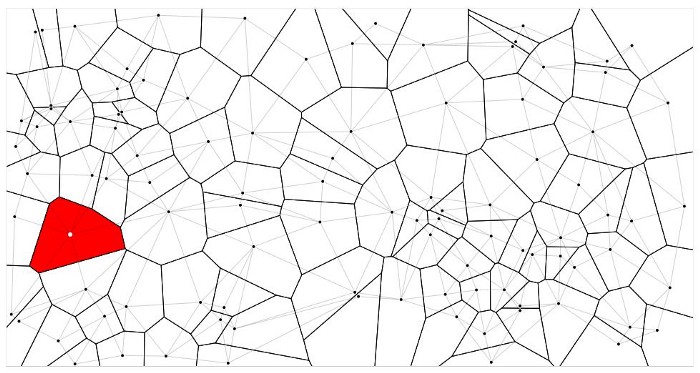
The most common form of visualization is the decision boundary, where the space that contains the data is marked to make the boundaries of each class clear. Veroni diagrams are another type of useful visualization, the diagram displays the area occupied by a point in relation to the distance to the other points, one can use this diagram to find the nearest neighbor of a new point by finding the polygon in which the unknown point lies.
Distance Metrics
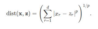
- The most common function is the Minkowski distance because it’s a generalization of other common functions such as euclidean and manhattan distance.
Shortcommings
- K must be set globally
- All points receive equal weights
- Slow on big datasets
- Since the method relies heavily of the distance function the method doesn’t perform well on high-dimensional data since the points of the same class tend to be distant2.
Curse of dimensionality on KNN
Assuming uniformly randomly distributed data in 3-D space in the form of a cube with edges equal to 1. To find the nearest neighbors one would need to define a point, find the high-dimensional structure that is around this point (a cube), and then find all the other points that are inside this smaller structure. The size of this structure can be easily calculated:
- l^d (l is the edge length and d is the number of dimensions) or k/n (n is the count of data points)
- By testing numbers on l^d = k/n we can see that with the increase of k the size of the small box starts to get almost to the size of the space. (you can check that easily by using n = 1000, d = [2, 10, 100, 1000] to see how l quickly approximates to 1 with the increase of dimensions).
This happens because the points are not close to each other at all in high dimensional spaces, consequently, the distance function stops being an appropriated metric. In high-dimensional spaces the points are almost equally as far away from each other and never in the center, always at the borders, making the use of KNN improper3.